
This article was written by guest author Thomas Murray. Ultiworld’s coverage of the 2016 Club Championships is presented by Spin Ultimate; all opinions are those of the authors. Please support the brands that make Ultiworld possible and shop at Spin Ultimate!
The purpose of this article is to outline an alternative method for ranking ultimate teams, allocating National Championship bids to the regions, and predicting single-game and tournament outcomes. At the end of this article, I report predictive probabilities derived from this method for each team’s pool placement and tournament finish at the National Championships this week. I will keep technical details in this article to a minimum. ((If you contact me at 8tmurray at gmail dot com, I would be happy to send you a PDF with the bare bones technical details. I will soon be submitting a manuscript to a statistical journal with these details and an objective evaluation of various methods for ranking ultimate teams.))
Like the current algorithm, the proposed method does the following:
- accounts for strength of schedule
- rewards teams for larger margins of victory
- decays game results over time, i.e., down-weights older results
- down-weighting shortened games, e.g., 10-7
- probabilistic bid allocation
- prediction
I think the current algorithm and bid allocation scheme are pretty darn good, and overall these tools/procedures have been beneficial for fostering a more competitive and exciting sport. Frankly, we are splitting hairs at this point with respect to ranking, and even bid allocation. The current algorithm doesn’t facilitate prediction, however. I am doing this because I enjoy this sort of thing, and minor improvements for ranking and bid allocation can still be worthwhile. The predictions are interesting in their own right.
I plan to maintain current rankings, and nationals predictions for all divisions in Club and College on my website.
Thank you Nate Paymer for making the USA Ultimate results data publicly available at www.ultimaterankings.net. This was an invaluable resource.
The Method
The key idea is that a win is split between the competing teams based on the score of the game. This is what I call the “win fraction.” In a win/loss model, the winning team gets a full win, or a win fraction of 1.0, and the losing team gets a total loss, or a win fraction of 0.0.
In the proposed method, the winning team gets a win fraction that depends on the proportion of goals that they scored and the losing team gets the remainder. The win fraction for the winning team is depicted in the figure below as a function of their proportion of the total points scored in the match.
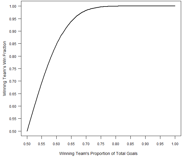
Note that there is a diminishing marginal return for larger margins of victory, just like the current algorithm, and in line with our subjective notions. ((I derived the win fraction through a working assumption about the point-scoring process. Namely, the win fraction reflects the % of games that a team would win against their opponent if their probability of scoring on each point is equal to p, and the game was played hard to 13. The observed win fraction in a particular game is calculated by plugging in for p the observed proportion of points that the team scored. This definition for the win fraction is a subjective choice, but I believe it is reasonable, and it results in a parsimonious and useful method.))
Using the win fractions, one can estimate a strength parameter for each team, just like a win/loss model. A point-scoring model also works similarly, but each team is attributed multiple “wins” each game equal to the number of points they scored. The major flaw of a point-scoring model is the marginal return for larger margins of victory is constant, rather than diminishing. The major flaw of a win/loss model is that it doesn’t use all the available information, and tends to perform poorly with small numbers of results like we deal with in ultimate. In particular, win/loss models vastly overrate undefeated teams that played an obviously weak schedule. The hybrid model alleviates both of these issues.
I also assign a weight to each match based on when it was played relative to the most recent week, and the winning score. I down-weight matches by 5% each week, and down-weight shortened matches in proportion to the amount of information they contain relative to a match played to 13. ((The above weights and win fractions for each match lead to an objective function, called the likelihood. I take a Bayesian approach, so I also specify the same weakly informative prior distribution for each team’s strength parameter. Doing so ensures the rankings are fair and dominated by the results from the season. Together the likelihood and prior results in a posterior distribution that tells me the likely values for the team strength parameters, and thus the likely rankings.))
Rankings
As is the case typically, although I cannot simply write down the posterior distribution in a tidy equation, I can draw lots of random samples from the posterior distribution and use these samples to learn about the team strength parameters. In particular, each sample from the posterior distribution corresponds to a ranking of the teams.
The actual rankings I report reflect each team’s average rank across all the posterior samples. For example, if Brute Squad is ranked 1st in 40% of the samples, and 2nd in 60% of the samples, then their average rank is 1.8 = 1*(0.4) + 2*(0.6). In contrast, if Seattle Riot is ranked 1st in 60% of the samples, and 2nd in 40%, then their average rank is 1.4 = 1*(0.6) + 2*(0.4). In this case, Seattle Riot would be ranked ahead of Brute Squad. Bayesian methods, sometimes called Monte Carlo methods, are quite popular, in part due to Nate Silver over at 538, and huge advancements in computational power and statistical methodology during past 25 years or so.
Probabilistic Bid Allocation
The current rank-order allocation scheme could still be used based on the rankings. However, this new method naturally facilitates an alternative probabilistic bid allocation scheme. To do this, I calculate the probability that a particular team is in the top 16 (or top 20) using the posterior samples.
By summing these probabilities for all the teams in a particular region, I calculate expected number of top 16 teams in that region, which I call the bid score. To allocate the 8 (or 10) wildcard bids, I sequentially assign a bid to the region with the highest bid score, subtracting 1 from the corresponding region’s bid score each time a bid is awarded. In this way, the bids are allocated to reflect regional strength, accounting for uncertainty in the actual rankings.
Prediction
Because the proposed method relies on the win fraction, which is derived from a working assumption between the probability that a team scores on a particular point and the probability they win the game, I can invert the strength parameters of the two teams into the average probability that one team scores on the other in a particular point, and then simulate a match between the two teams using the resulting point scoring probability.
Extrapolating, I can simulate the entire National Championships in each division. In particular, I can sample one set of strength parameters for the 16 teams competing at nationals, simulate the tournament given these values, and record each team’s finish. Iterating this process, I can calculate the posterior probability of each teams pool placement and finishing place, i.e., 1st, 2nd, semis, and quarters.
Results
Below, I report the top 25 teams in each division at the end of the regular season, along with bid allocation under the two schemes. I then report the predictive probabilities of each team’s placement in their pool, and Nationals finish at this week’s tournament.
Men's: End Of Regular Season Rankings & Bid Allocation
[table id=646 /][table id=649 /]
Mixed: End Of Regular Season Rankings & Bid Allocation
[table id=648 /][table id=650 /]
Women’s: End Of Regular Season Rankings & Bid Allocation
[table id=647 /][table id=651 /]
Men's Probabilities
Pool A[table id=659 /]
Pool B
[table id=660 /]
Pool C
[table id=661 /]
Pool D
[table id=662 /]
Championship Bracket
[table id=658 /]
Mixed Probabilities
Pool A[table id=664 /]
Pool B
[table id=665 /]
Pool C
[table id=666 /]
Pool D
[table id=667 /]
Championship Bracket
[table id=663 /]
Women's Probabilities
Pool A[table id=652 /]
Pool B
[table id=653 /]
Pool C
[table id=654 /]
Pool D
[table id=655 /]
Championship Bracket
[table id=657 /]
Originally published at: https://ultiworld.com/2016/09/28/nationals-probabilities-every-teams-chances-to-win-a-title/